🛑 Don't Stop 'til You Get Enough — Reintroducing the “Precision is the Goal” Stopping Criterion, and Making It Decisive ⚖️

Know when you have enough data, and when a null result is a real finding. Interactive simulations and a calculator included. 🕹️⏯️🧮

“How much data is required?”

This is one of the most common questions in hypothesis and A/B testing, and it can be asked at two different moments.

Before any data is collected, it is a planning question. The standard answer is a power analysis: supply a minimum effect size and how often you are willing to be wrong in each direction, and out comes a sample size. It is a sensible place to start. But what if the true effect is much stronger than you assumed, and you could have stopped weeks earlier? Or what if, halfway through a clinical trial, a treatment shows signs of doing harm?

The more flexible alternative is to check as the data arrives, known as sequential hypothesis testing, or sequential testing for short. It asks a different question:

“Have we collected enough data yet?”

As tempting as sequential hypothesis testing is, it has a well-known failure mode. Peek often enough, and sooner or later an early, unrepresentative stretch of data will meet the stopping rule. In most standard methods that same rule also decides the verdict, so the experiment stops precisely when the data happen to look most convincing. The result is a form of confirmation bias: the data appear to confirm a finding that is really just a lucky fluctuation, and no ill intent is needed for it to happen. Why this happens is well understood, and it can be corrected for.

That correction is the focus of this post: a rule that tells you when you can confidently stop an experiment already under way. A welcome side effect is that error rates stay low, and when there truly is no meaningful difference, you can say so, accepting the null hypothesis with near-zero false rejections. A companion post will show that the same machinery also works before a study starts, to plan how much data to collect in the first place.

This post is for anyone who runs experiments and has to decide both when to stop them and how to interpret the result: A/B testers, analysts, data scientists, researchers, and anyone who has ever stared at a dashboard wondering whether today is the day to call it.

No prior knowledge of Bayesian statistics is required, just a basic understanding of probabilities. If you have a rough idea of what a p-value is, you already know more than enough. (If you don’t, that’s fine too — and it may save you some unlearning of common p-value misreadings.)

By the end you will be able to:

• 🛑 Tell stopping apart from deciding ⚖️, and see why using one rule for both turns lucky streaks into false verdicts, even with the Bayesian tools often pitched as the fix.
• 📏 Quantify what counts as “close enough” to the null hypothesis (the “no effect” baseline), and hold to it, rather than letting the effect size you planned around (in A/B testing, your minimum detectable effect, or MDE) be quietly forgotten between the planning meeting and the write-up.
• ✅ Accept the null hypothesis, instead of awkwardly failing to reject it, whenever “no meaningful difference” is the finding you actually need.
• 🎯 Stop on precision (how narrow your uncertainty has become) rather than on the verdict, using John Kruschke’s Precision is the Goal, plus a small tweak of mine that makes it reliably conclusive.
• 💰 See why precision costs data, and check whether you have enough, and if not, how much more you need; the companion post takes this further into full study planning.

Along the way you can play with two interactive simulations 🕹️⏯️ and try a calculator on your own data 🧮.

If you are already comfortable with posteriors, HDIs and ROPEs, the main thread will feel slow in places, and the short appendices after the summary go a little further.

For the full technical treatment, I have also written this up as an arXiv preprint. You won’t need it to follow along, but it is there as a reference for the finer details.

🎬 Prelude: What I’m Talking About When I Talk About Accepting the Null

Most of us learned hypothesis testing as a hunt for differences. Before we look at how experiments end in practice, let’s add a tool that’s often missing from the kit: a way to conclude that there is no difference worth acting on. Sometimes that is exactly the finding you need:

• 💻 Do no harm. A new release, a refactor, cheaper infrastructure or an updated model should not hurt a key metric such as conversion, latency or accuracy.
• 💊 Generic drugs. A generic must be shown to work like the brand-name drug, within margins set by regulators.
• 📋 Futility. A programme or trial is stopped once it is clear that its effect, if any, is too small to be worth pursuing.

A standard significance test cannot deliver this. It can only reject the null hypothesis or, awkwardly, “not reject” it, and not rejecting may simply mean too little data: absence of evidence is not evidence of absence.¹ To conclude that there is no difference worth acting on, rather than none at all, you first need to decide what counts as “close enough”. And as we’ll see, that same decision also changes when you can safely stop collecting data.

How Experiments Actually End

How did your last experiment actually end?

In large-scale A/B testing, results are typically watched as they come in, and a test is stopped once a heuristic, such as a p-value, a confidence interval or a Bayes Factor, crosses a predetermined threshold.²

Scientific research mostly runs the other way round.³ The sample size is fixed in advance, usually by a power analysis, and the study runs to the end. Its characteristic failure arrives later, once the data is in: the minimum effect size that went into the planning calculation appears nowhere in the heuristics that are reported, so it quietly drops out of the conclusion.⁴ That second failure is the subject of the companion post. This one is about the first: continuous monitoring.

One Heuristic, Two Jobs

The most popular heuristic by far is the p-value, from the Null Hypothesis Significance Testing framework (NHST). Briefly, the p-value quantifies how surprising the data would be if the null hypothesis were true.

Used as a stopping rule in sequential testing, it means recalculating the p-value as the data comes in, until it falls below an agreed threshold, usually 0.05 and sometimes stricter. That same threshold is also the decision rule: once the p-value is below it, the null hypothesis is rejected. The same is true of other heuristics, such as Bayes Factors: the thresholds differ, but stopping and deciding remain one and the same.

In other words, the heuristic that signals when to stop collecting data is the same one that delivers the verdict. The experimenter stops because the result has turned “statistically significant”, and many will unwittingly conclude that it is also meaningful.

“Statistically Significant” Does Not Imply Meaningful

A common misconception is to confuse “statistical significance” with a meaningful outcome. A p-value below the threshold says only that the data would be unlikely if the null hypothesis were true. It says nothing about whether the difference is large enough to matter.

Think of a researcher asking whether a therapeutic works differently for men and women, who finds it beneficial in 72.1% of one group and 72.3% of the other. With enough patients, even that 0.2 percentage point gap will become “statistically significant”, whether judged by a p-value or a Bayes Factor. In practice, however, no clinician would prescribe differently because of it. Why does a gap that small cross the threshold? With more data the estimate becomes ever more precise, so even a tiny but real departure from the null eventually produces a p-value below the threshold. You’ll be able to see this for yourself in the Snapshot Explorer further down, with its p-value rejects, ROPE accepts button.

The key takeaway is that a deviation from the null hypothesis should be large enough to justify acting on it, for example by changing the status quo.

Tiny real effects are one way a p-value can mislead. Repeated looking is another, and it misleads even when there is no effect at all, as the simplest sequential hypothesis test shows: a fair coin toss.

NHST Catastrophically Fails the Fair Coin Test

[Title options to choose from: “Peeking at P-Values: The Fair Coin Test” · “The Fair Coin Test: Where Peeking Goes Wrong” · “Peek Long Enough, and a Fair Coin Looks Loaded” · “A Fair Coin, an Impatient Analyst, and the P-Value”]

The beauty of tossing a virtual fair coin is that we know the ground truth, which makes it a useful testbed for any hypothesis-testing mechanism, sequential or otherwise. For a fair coin, the null hypothesis that it is fair should be accepted; for a heavily loaded coin, the same null hypothesis should be rejected.

The first limitation of NHST shows up straight away: the p-value carries no information for accepting the null (for details see the appendix on why p-values cannot accept the null). For a fair coin, the best it can offer is the awkward double negative of “not rejecting” it. We will later meet Bayesian mechanisms that can accept the null.

But even if we settle for NHST’s ability to reject, it fails the sequential fair coin test badly. To see this, we simulated 200 fair coin sequences of 30,000 tosses each, and peeked at the p-value after every toss:

• If p < 0.05, we stop collecting data and reject the null hypothesis, incorrectly, since the coin is fair.
• If p ≥ 0.05, we do not reject it (an inconclusive outcome) and toss again.

How often should we expect to wrongly reject a fair coin? Naïvely, 5% of the time, as per the threshold. That is true for a single look. But every look is another chance for a random fluctuation to dip below 0.05, and over many looks those chances add up.

The figure below shows the cumulative decision rates as the tosses accumulate: rejections in red and non-rejections in gray, summing to 100% at every point. Once a sequence is rejected it stops, so its rejection is carried forward to every later toss.

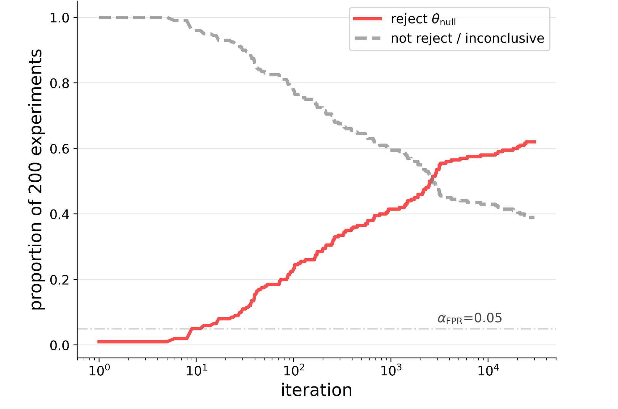
Cumulative decision rates for 200 fair coin sequences when the p-value is used both to stop and to decide (note the logarithmic x-axis). The dash-dotted line marks the nominal 5% false positive rate. The code is in this notebook.

The false rejection rate, otherwise known as the false positive rate, climbs far past the nominal 5%: to about 20% within the first hundred tosses, and to over 60% by 30,000. And it keeps climbing. Under a true null hypothesis the p-value wanders between 0 and 1 as tosses accumulate, and given enough looks it eventually wanders below any threshold.

John Kruschke, author of Doing Bayesian Data Analysis, demonstrated this vividly for the fair coin, and summed it up with a quip:

“With infinite patience, NHST results in 100% false alarms.”

A natural first fix is a Bayesian heuristic that can accept the null hypothesis, such as the Bayes Factor. It turns out not to be enough: used both to stop and to decide, it runs into the same confirmation bias. In Kruschke’s fair coin simulations it falsely rejected the null about 20% of the time, and for a loaded coin with a true rate of 0.65 it falsely accepted the null about 40% of the time, what is known as a false negative (see the appendix on Bayes Factors).

The root issue is shared by the p-value and the Bayes Factor alike: the heuristic that decides is also the one that stops.

🛑 Gotta Keep ‘em Separated ⚖️

The fix is to keep the two jobs apart, by giving each its own heuristic. Using one heuristic for both is convenient, but it is exactly what lets a statistical fluke through: given enough looks, a chance fluctuation will eventually cross the line, and the experiment stops right there, with a verdict to match.

It’s like letting whichever team happens to be ahead decide when the game ends. In sport, the end is set by a rule agreed before the game starts, such as the clock in basketball or the target score in volleyball, however the game happens to be going at any given moment.

The principle, then, is that the stopping rule must never be the verdict alone. (We’ll see later that the two can be recombined, carefully.) In the approach we’ll explore:

• 🛑 Stopping depends on how certain we are about the parameter, regardless of where its estimate sits relative to the null.
• ⚖️ Deciding depends on where the estimate sits relative to a “close enough” region around the null, agreed in advance.

To make both precise, we first need two key properties of a posterior: its width and its location.

The HDI: A Posterior’s Width and Location

Everything the data tells us about a parameter is held in its posterior distribution $p(\theta \mid {\rm data})$ : how plausible each possible value is, given what we have observed so far. Two of its properties do most of the work in hypothesis testing:

• Width: how uncertain we still are. A wide posterior means many values remain plausible, a sign we may not have collected enough data.
• Location: where the plausible values sit, which we can compare to the null value.

These map neatly onto the separation above: width will drive the stopping rule, and location the decision rule.

To get a feel for both, let’s watch a posterior narrow as data piles up, using one of the most famous weaknesses in basketball: the free throws of Shaquille O’Neal. Shaq dominated play close to the basket for nearly 20 years, but was so unreliable from the line that opposing teams fouled him on purpose, a tactic known as Hack-a-Shaq.⁵ A free throw either goes in or it doesn’t, so it behaves like the toss of a (possibly loaded) coin: the same binomial data as a conversion in an A/B test, or a defective item coming off a production line.

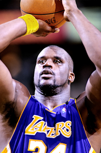
Shaq at the free throw line for the Los Angeles Lakers, 1999. Photo: Steve Lipofsky, Basketballphoto.com, CC BY 3.0.

The figure below shows the posterior of his free throw success rate $\theta$ from two data sets: the 2004/5 season, with 765 attempts in 73 games (left), and his full career, with 11,252 attempts in 1,207 games (right).

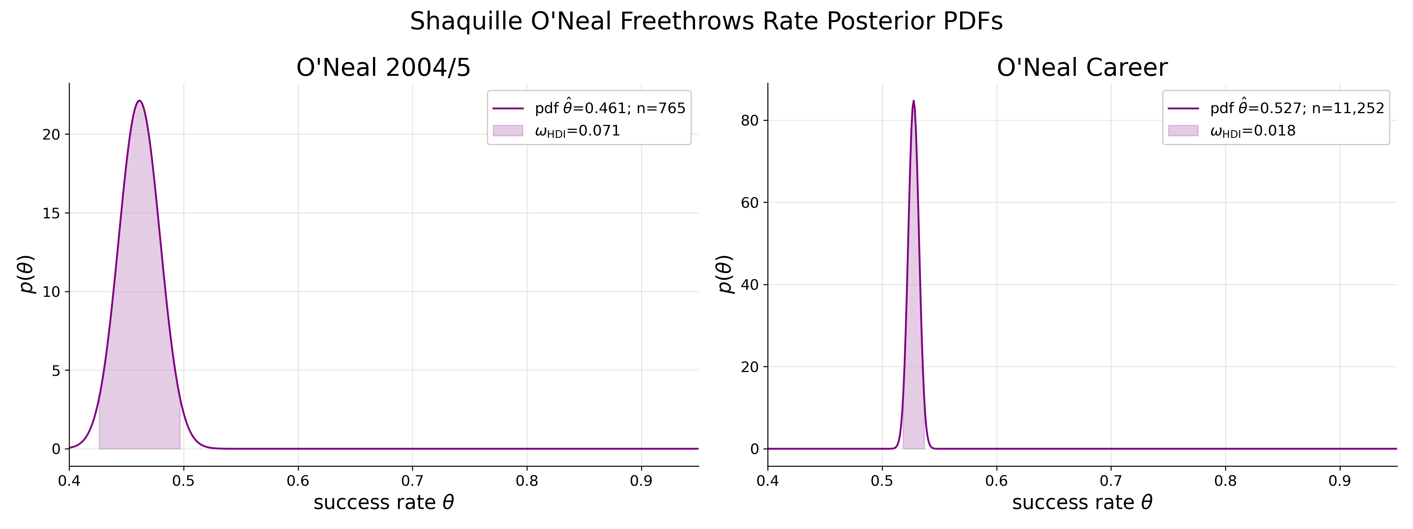
Posteriors of Shaq’s free throw success rate. Shaded areas are the 95% HDIs and the dashed line marks 50%. Left: the 2004/5 season (765 attempts). Right: his full career (11,252 attempts). About fifteen times the data gives a posterior about four times narrower.

The higher a curve at a given value, the more plausible that value is as Shaq’s true, underlying success rate.

The shaded region is a credible interval, the Bayesian counterpart of the frequentist confidence interval,⁶ marking where most of the posterior lies. Throughout this post we use 95% of it. There are several ways of choosing which 95%, and we use the Highest Density Interval (HDI). Picture a horizontal waterline slowly lowered from the peak of the curve: the HDI is the stretch between the two points where the line crosses the curve, at the moment the area beneath it first reaches 95%. Every value inside the HDI is therefore more plausible than any value outside it. (See the preprint’s Appendix A for a formal definition.)

An HDI is summarised by its two boundaries, $\rm HDI_{min}$ and $\rm HDI_{max}$ , which give its location, and by the distance between them, which gives its width:

\(\omega_{\rm HDI} \equiv {\rm HDI_{max}} - {\rm HDI_{min}}\)

Width: More Data, More Certainty

The most striking difference between the two panels is their width: $\omega_{\rm HDI}=7.1\%$ for the single season, against $1.8\%$ for the full career. Roughly fifteen times as many attempts produced a posterior roughly four times narrower.

That is no coincidence: the width shrinks in proportion to $1/\sqrt{N}$ , where $N$ is the sample size, and $\sqrt{15} \approx 3.9$ . This is the precise sense in which more data means more certainty, and it comes with a price tag: halving the width takes four times the data. We’ll return to that price later on.

Note that the width says nothing about where the posterior sits, only how sure we are of it. That is exactly the property a reliable stopping rule needs.

Location: Where the Plausible Values Sit

The location is read off the HDI boundaries. For Shaq’s 2004/5 season freethrow rate the HDI spans 42.6%–49.7%: given that season’s data, there is a 95% probability that his underlying success rate lay within this range. For his career it spans 51.8%–53.7%.⁷

These numbers invite a question:

“Was Shaq’s free throw ability better or worse than the toss of a fair coin?”

The career panel answers better, but only slightly: by about 2.7 percentage points, give or take one. With 11,252 attempts, though, even a far tinier departure from 50% would have been told apart from it. The more useful question is:

“Was Shaq’s free throw ability meaningfully better or worse than the toss of a fair coin?”

To answer it, we first have to decide what “meaningful” means.

📏 Quantifying “Close Enough”

If Shaq’s underlying rate was $\theta=0.501$ , would you consider it practically a fair coin toss? How about 0.51? Or 0.53? At the end of the day this is a subjective call, and that’s fine. Part of analysing data is being aware of making such calls, as long as one can justify them.

For argument’s sake, let’s say that any success rate between 45% and 55% is practically a fair coin toss, and redraw Shaq’s career posterior with these boundaries as a gray band.

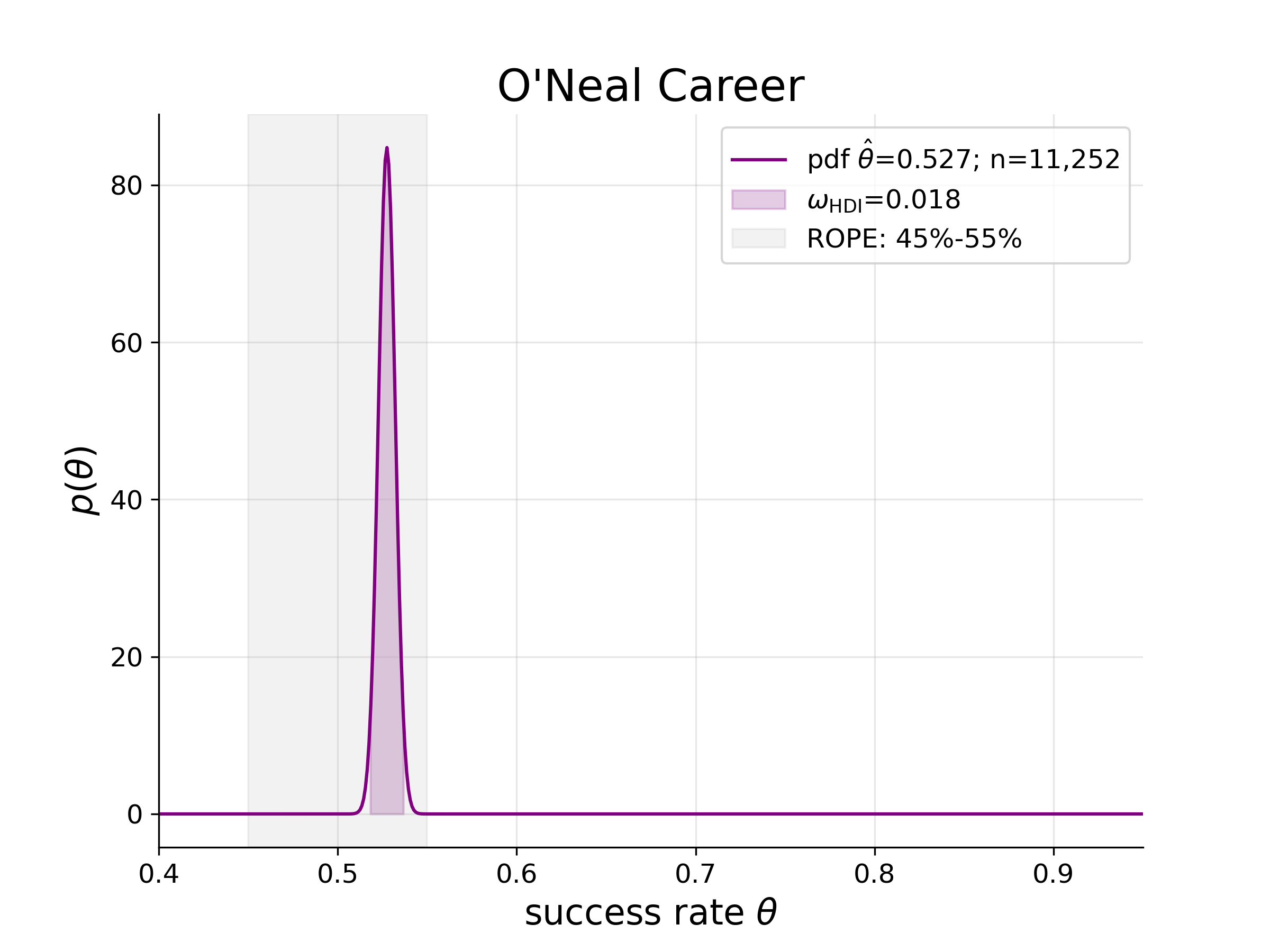
Shaq’s career posterior. The gray band marks 45%–55%, the success rates we consider practically a fair coin toss. The HDI (shaded) sits entirely inside it.

The career HDI, 51.8%–53.7%, sits entirely within the band. So, for all practical purposes, Shaq’s free throw success was like a fair coin toss. (We chose the band here after seeing the data. In a real experiment the order must be the other way round, as we’ll see shortly.)

The same question arises in every experiment: what change is large enough to be worth acting on? A meaningful effect is one large enough to justify a real-life decision, so which effects qualify depends on the decision. What we need is a way to state that, and to state it in advance.

The ROPE: Committing to “Close Enough” in Advance

[Subheading options to choose from: “ROPE: Drawing the Line Before the Data Arrives” · “The ROPE: Where ‘No Difference’ Lives” · “Region of Practical Equivalence: Naming What Doesn’t Matter” · “ROPE: A Minimum Effect Size You Can Actually Hold To”]

The gray band has a name: the Region of Practical Equivalence, or ROPE. It is a region around the null value, wide enough to hold every value we would consider no meaningful change. If the truth sits anywhere inside the ROPE, the honest report is that nothing meaningful happened. Given its boundaries $\rm ROPE_{min}$ and $\rm ROPE_{max}$ , its width is $\omega_{\rm ROPE}\equiv \rm ROPE_{max} - ROPE_{min}$ .

How wide should the ROPE be? There is no general answer, and that is the whole point: the width is the domain-specific question of what a meaningful minimal effect size is.

Consider a dice manufacturer with two clients. A board-game publisher such as Hasbro, makers of Monopoly, needs dice fair enough that no player notices a bias. A casino needs dice fair enough to satisfy a gaming regulator, a far stricter standard. Testing a batch amounts to rolling and counting sixes, a binomial experiment whose null value is a probability of 1/6 ≈ 16.7%.⁸ Same factory, same dice, same test, yet the casino’s ROPE around 1/6 has to be much narrower than Hasbro’s, and a batch may be practically fair for one client and not for the other.

So the ROPE boundaries are not computed but chosen, before any data arrives, from what we already know about the domain. That is the discipline of it: we commit to what counts as a meaningful change while the result is still unknown, so that the commitment cannot later be shaped by the result it is meant to judge. (For established ways of choosing a ROPE, see the appendix on choosing a ROPE in practice.)

With both the HDI and the ROPE in hand, we can put them together: first their locations, into a decision rule, and then the HDI’s width alone, into a reliable stopping rule.

⚖️ The HDI+ROPE Decision Rule

We have already seen one decision in action: Shaq’s career HDI sat entirely within the ROPE, so we concluded that his free throws were, for all practical purposes, a fair coin toss. Let’s generalise. The HDI+ROPE decision rule compares the location of the HDI with that of the ROPE, and the outcome is either conclusive or inconclusive.

Conclusive Outcomes

The conclusive outcomes are easiest to see in an illustration:

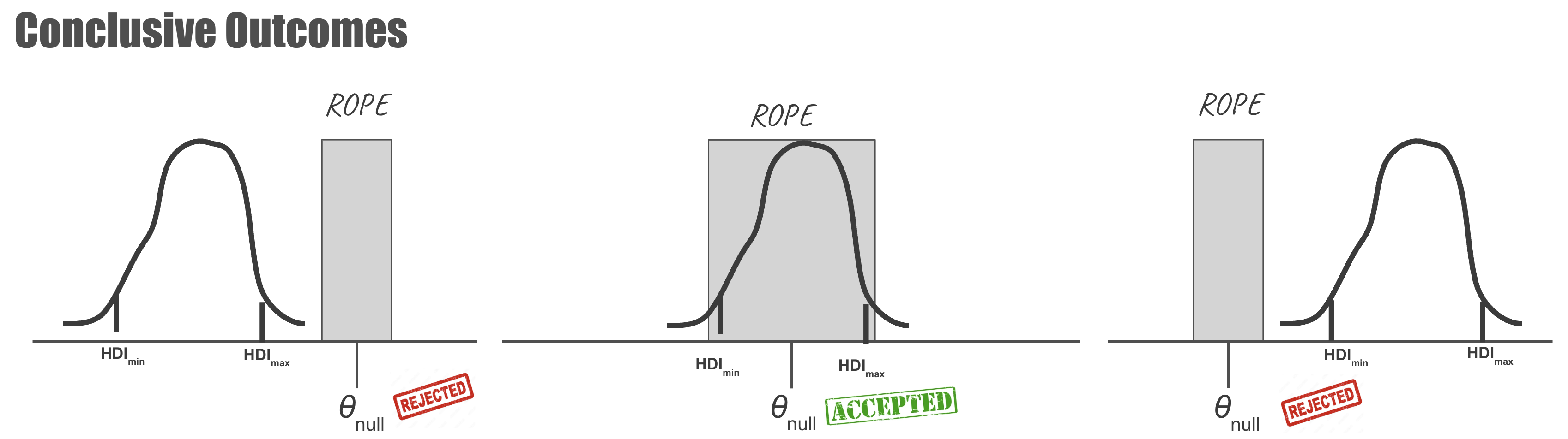
The three conclusive outcomes. Curves are posteriors, with ticks marking the HDI boundaries; gray boxes are the ROPEs around the null value. Left and right: the HDI is entirely outside the ROPE, so the null is rejected. Centre: the HDI is entirely inside the ROPE, so the null is accepted.

Two of these outcomes reject the null hypothesis and one accepts it:

• ✅ Accept the null: the HDI is completely inside the ROPE, ${\rm ROPE_{min}} \le {\rm HDI_{min}} \lt {\rm HDI_{max}} \le {\rm ROPE_{max}}$ .
• ❌ Reject the null: the HDI is completely outside the ROPE, on either side, ${\rm HDI_{max}} < {\rm ROPE_{min}}$ or ${\rm ROPE_{max}} < {\rm HDI_{min}}$ .

Note that accepting the null can be a finding in its own right, rather than a failure to detect something. This is exactly what the p-value could not offer.

Inconclusive Outcomes

The three remaining outcomes are all inconclusive:

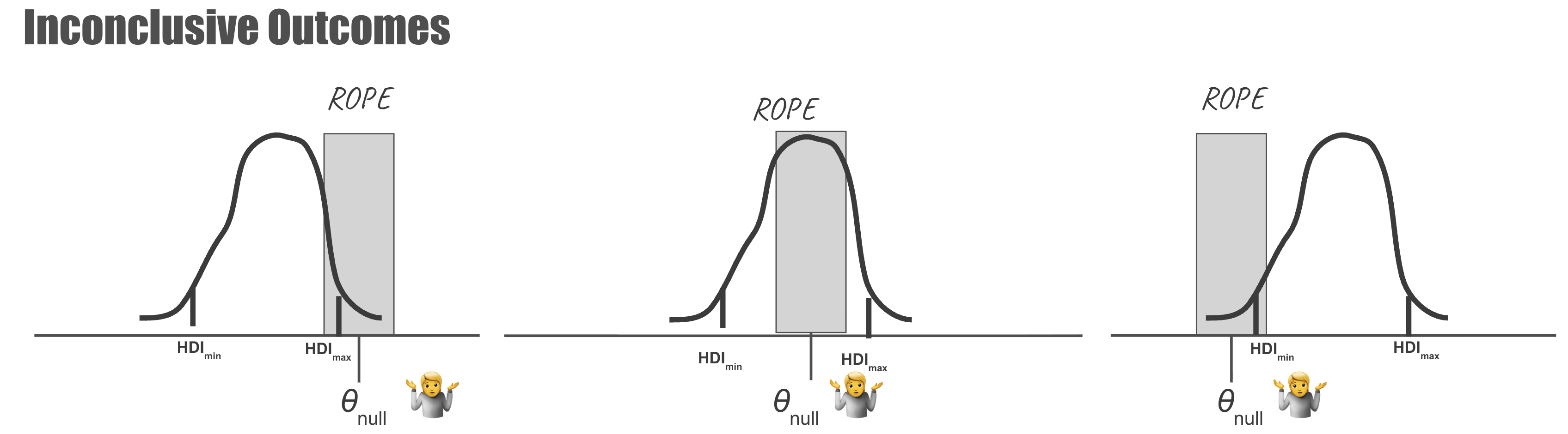
The three inconclusive outcomes. Left and right: the HDI crosses one ROPE boundary. Centre: the HDI is wider than the ROPE and spills over both boundaries.

They share one feature:

• 🤷 Inconclusive: the HDI straddles at least one ROPE boundary, sitting partly inside and partly outside.

The centre panel is worth a closer look. Its HDI is wider than the ROPE, $\omega_{\rm HDI} > \omega_{\rm ROPE}$ , so wherever it sits it can never fit inside it. Where it is now, it can neither accept nor reject. Shifted well away from the null, a posterior this wide could still reject, but it can never accept. In other words, being able to say “no meaningful difference” requires an HDI narrower than the ROPE, a point we’ll return to when deciding when to stop.

What to do with an inconclusive result depends on the experiment’s budget. If more data can be collected, it narrows the HDI and may well resolve the straddle. If the budget is spent, a decision can still be forced, but it then becomes a risk assessment that weighs the cost of being wrong in each direction, which is domain specific and beyond the scope of this post.⁹ Much of the rest of this post is about the first option: when to keep collecting, and when it is safe to stop.

One Fair Coin, Three Verdicts

The cartoons above are idealised. To see the decision rule on real binary data, let’s return to the virtual fair coin from earlier, where we know the truth: $\theta_{\rm true}=0.5$ . We use the same ROPE as for Shaq, [45%, 55%], and follow a single sequence of tosses. This sequence was randomly generated but then hand-picked, because it shows all three outcomes.¹⁰ (Claims about how often each outcome happens will come later, from 5,000 sequences.)

Here is the posterior at three points along the same sequence:

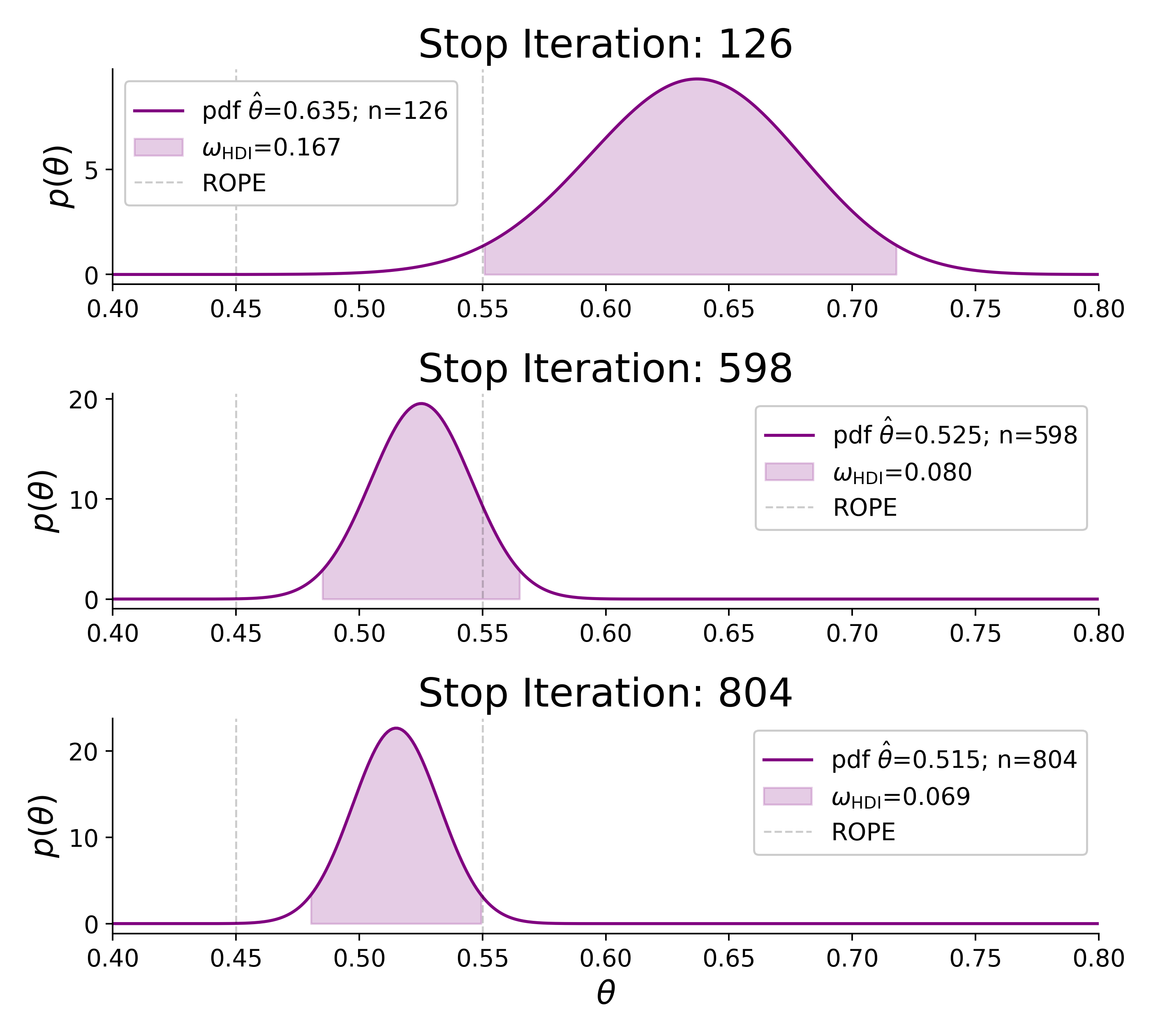
Posteriors of one fair coin sequence after 126, 598 and 804 tosses. Shaded areas are the 95% HDIs; vertical dashed lines mark the ROPE boundaries.

• After 126 tosses: $\hat\theta=0.635$ , and the HDI spans 0.551–0.718, entirely above the ROPE. ❌ Reject the null, just like the right-hand conclusive cartoon, even though this HDI ($\omega_{\rm HDI}=0.167$ ) is wider than the ROPE.
• After 598 tosses: $\hat\theta=0.525$ , and the narrower HDI ($\omega_{\rm HDI}=0.080$ ) straddles the upper ROPE boundary. 🤷 Inconclusive.
• After 804 tosses: $\hat\theta=0.515$ , and the HDI spans 0.480–0.549, entirely inside the ROPE. ✅ Accept the null, if only by a hair (0.549 against a boundary of 0.55).

Same coin, same tosses, three different verdicts. The only thing that differed was when we stopped to look. Which raises the question this post is really about: when should we stop? Before we get there, the verdicts above deserve a closer look.

What Exactly Are We Accepting/Rejecting?

When a verdict comes in, it is tempting to read it as a verdict on the sample value. It isn’t.

After 804 tosses we accept the null, $\theta_{\rm null}=0.5$ , not the sample value of 0.515. What we are accepting is that the true rate is practically equivalent to 0.5, within the ROPE we committed to.

After 126 tosses we reject the null, but that is not an endorsement of 0.635. Here the point is sharper, because we know the true value is 0.5, and it isn’t even inside the HDI. Rejecting the null says only that the plausible values sit meaningfully away from it.

The decision rule accepts or rejects the null value, not the sample value.

That 126-toss verdict was also simply wrong, which brings us to the two ways a conclusive verdict can be incorrect:

• A false reject: we reject the null although the true value lies inside the ROPE. This is what is usually called a false positive (or Type I error), just named more literally, with the null now a region rather than a single point.
• A false accept: we accept the null although the true value lies outside the ROPE. This is the false negative (or Type II error) idea, with one difference: a classic false negative merely fails to reject a false null, whereas a false accept actively accepts it.

An inconclusive verdict, by contrast, is never wrong. It just isn’t a verdict yet.

Three Stopping Algorithms

So far we have used the HDI and the ROPE to decide on a verdict once we look at the data. Now back to the question we left hanging, and the key question of sequential testing: when should we stop collecting?

The three snapshots of our fair coin, at 126, 598 and 804 tosses, were not picked at random. Each is where one of three stopping algorithms stops, which we now introduce: HDI+ROPE, Precision is the Goal (PitG), and Decisive Precision is the Goal (DPitG). All three share the HDI+ROPE decision rule above and differ only in when they stop:

Algorithm	🛑	⚖️	Logic
HDI+ROPE	Conclusive?		Location only
Precision is the Goal (PitG)	$\omega_{\rm HDI} \le \omega_{\rm goal}$	Conclusive?	Precision then Location
Decisive PitG (DPitG)	($\omega_{\rm HDI} \le \omega_{\rm goal}$) & (Conclusive)		Precision and Location

The three stopping algorithms. 🛑 marks the stop criterion and ⚖️ the decision rule. “Conclusive” means the HDI is completely inside or outside the ROPE; $\omega_{\rm HDI} \le \omega_{\rm goal}$ means the HDI is at least as narrow as a precision goal set in advance.

In short, HDI+ROPE stops on location alone, PitG stops on width and only then looks at location, and DPitG requires both at once. Each of the following subsections fills in one row of the table.

🛑 HDI+ROPE: Stop When Conclusive

The simplest algorithm keeps collecting until the decision rule gives a conclusive outcome,¹¹ then stops and reports it: once the HDI is fully outside (or inside) the ROPE, it rejects (or accepts) the null. Like the p-value and the Bayes Factor, it uses a single criterion both to stop and to decide.

On our hand-picked fair coin it stops at toss 126 (top panel of the three snapshots) and wrongly rejects the null 🤥. An early run of heads was enough to push a still-wide HDI past the ROPE, and the algorithm took the bait. This is the same confirmation bias we saw with the p-value, now in Bayesian form.

What we need is a reason to stop that does not consult the verdict. The HDI’s width is exactly that.

🛑 Precision is the Goal: Stop When Narrow Enough

John Kruschke’s PitG gives the two jobs to two different heuristics: the stopping rule looks only at the width of the HDI, and the decision rule is applied only once data collection has stopped.

We set a precision goal $\omega_{\rm goal}$ in advance and, after each toss, compare the HDI width to it:

• $\omega_{\rm HDI} \le \omega_{\rm goal}$ : criterion met. Stop, then apply the decision rule.
• $\omega_{\rm HDI} > \omega_{\rm goal}$ : not met. Continue collecting (or, if the budget is spent, conduct a risk assessment).

Following Kruschke’s original analysis we use $\omega_{\rm goal}=0.08$ . It is narrower than the ROPE ($\omega_{\rm ROPE}=0.1$ ), as it must be: as we saw earlier, an HDI wider than the ROPE can never accept the null.

The key difference from HDI+ROPE, and from the p-value and the Bayes Factor, is that PitG monitors the posterior’s width rather than its location. A lucky streak can shift where the posterior sits, but it barely changes how wide it is, so there is no early, extreme moment for the stopping rule to pounce on. In his fair coin simulations, Kruschke found that PitG made zero false rejections across 1,000 sequences, as it also does in the 5,000 sequences we’ll see below. And because it does not stop on extreme runs, the sample value at the stop is also more accurate, including for loaded coins.¹²

🤷 Precision Isn’t Enough

Our hand-picked coin already shows the catch. PitG stops at toss 598 (middle panel of the three snapshots), where the precision goal is met, but the HDI straddles the ROPE, so the verdict is inconclusive.

This is not a quirk of one sequence. In Kruschke’s own fair coin figure, which I have reproduced, it is the most common outcome: more often than not, PitG stops with an inconclusive verdict. He mentions it only in passing, noting that PitG “did remain undecided in some cases”.¹³ In other words, PitG rarely says anything wrong, but often says nothing at all.

A small tweak, it turns out, resolves most of this, at the cost of a little more data.

🛑 Decisive Precision is the Goal: Stop When Narrow Enough and Conclusive

The tweak is to make the stopping rule a little more conservative. Instead of STOP THEN DECIDE, DPitG does STOP AND DECIDE:

Collect data until $\omega_{\rm HDI} \le \omega_{\rm goal}$ and the HDI is completely inside or outside the ROPE.

Once both criteria are met, the HDI+ROPE decision rule applies as usual. Until then the result is inconclusive: if the budget permits, data collection continues; otherwise one must resort to a risk assessment.

The figure below shows the difference. It is similar to the cartoons above, but the yellow box around each posterior has the width of $\omega_{\rm goal}$ , so an HDI that fits inside it meets the precision goal.

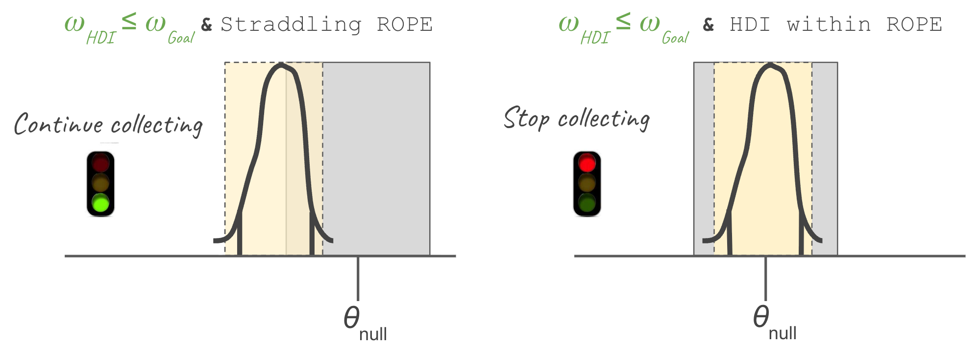
Two DPitG scenarios. In both, the HDI fits inside the yellow dashed box of width $\omega_{\rm goal}$ , so the precision goal is met. Left: the HDI straddles the ROPE, so DPitG keeps collecting. Right: the HDI is fully inside the ROPE, so DPitG stops and accepts the null.

In both panels the precision goal is met. On the left the HDI straddles the ROPE: PitG would stop here with an inconclusive verdict, whereas DPitG keeps collecting. On the right the HDI is fully inside the ROPE, and DPitG stops and accepts the null. These are two of eleven possible scenarios.¹⁴

On our hand-picked coin this means carrying on past toss 598, where PitG stopped, until toss 804 (bottom panel of the three snapshots), where the HDI is both narrow enough and inside the ROPE, and the null is correctly accepted.

DPitG is thus a hybrid of the other two: PitG’s precision criterion and HDI+ROPE’s conclusiveness criterion. This is the careful recombination promised earlier, since its stopping rule depends on whether the data can support a verdict, never on which verdict it is. Because precision must be met first, it never stops on an early lucky streak; and because it also requires a conclusive outcome, it rarely ends with nothing to say.

🕹️ Snapshot Explorer

▶️ Try it yourself. The Snapshot Explorer below shows a single look at a coin’s tosses. Drag the number of tosses and the share of heads, and watch the posterior, its HDI and the decision rule respond, together with what each stopping rule would do if this were the moment you looked. The p-value’s verdict is included for comparison. The buttons jump to the three snapshots of our hand-picked coin, and to a few extreme cases worth a look.

More Lessons from the Fair Coin Test

The Snapshot Explorer shows a single look at the data. To see how the three algorithms actually behave as the data accumulates, let’s follow coins through time: first our hand-picked one, toss by toss, and then 5,000 of them.

One Coin, Toss by Toss

We start with our hand-picked sequence, now following it toss by toss rather than at three snapshots, with the precision goal at $\omega_{\rm goal}=0.08$ as before.

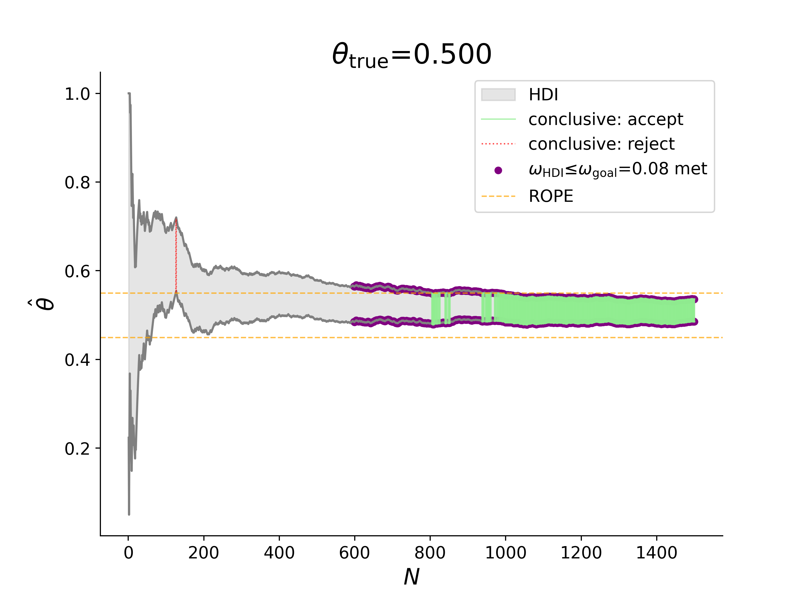
The 95% HDI (gray band) of our hand-picked fair coin sequence after each toss. Orange dashed lines: the ROPE boundaries. Red line: the HDI is fully outside the ROPE. Green: fully inside it. Purple dots: the precision goal is met.

Reading from left to right, all three stops sit on one timeline. At toss 126 an early run of heads pushes the HDI above the ROPE, and HDI+ROPE stops and wrongly rejects. At toss 598 the purple dots appear: the precision goal is met, so PitG stops, but the HDI still straddles the ROPE and its verdict is inconclusive. DPitG carries on until toss 804, the first point at which the HDI is both narrow enough and inside the ROPE, and correctly accepts.

Notice that the green does not stay on once it appears: just after 804 the HDI drifts back across the boundary a few times before settling inside it. An accept can come and go, and DPitG stops at the first one.

⏯️ Sequence Simulator

▶️ Try it yourself. The Sequence Simulator below replays the same hand-picked coin, toss by toss. Press Play / pause to watch it again, New random run for a fresh coin, Find a false reject to search random fair coins until HDI+ROPE wrongly rejects one, or Find a PitG inconclusive to see PitG’s catch; Our hand-picked coin brings you back. Narrow the precision goal and both precision-based rules wait longer; widen it towards the ROPE’s width and PitG ends inconclusive more often. And raise the true rate above 0.55, and rejecting becomes the correct answer.

As mentioned before, the hand-picked sequence was chosen because it shows the three algorithms reaching different outcomes. To see how often each outcome actually happens, we need many sequences.

5,000 Fair Coin Sequences

We now generate 5,000 fair coin sequences, each with a budget of up to $N_{\rm max}=1{,}500$ tosses, and run all three algorithms on every one of them. The figure below shows the resulting decision rates as the tosses accumulate. As with the p-value figure earlier, the rates are cumulative: once a sequence stops, its verdict is carried forward to every later toss. Since the coin is fair, accepting the null is the correct outcome and every rejection is a false one.

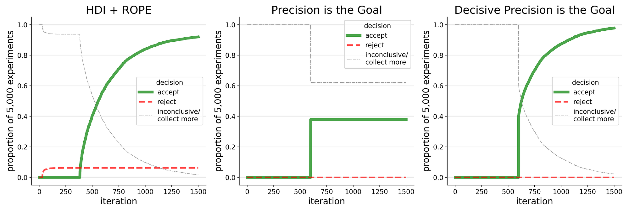
Cumulative decision rates for 5,000 fair coin sequences under each stopping algorithm. At every toss count the shares that have accepted the null (green solid), rejected it (red dashed) or are still inconclusive (gray dot-dashed) sum to 100%. Since the coin is fair, every rejection is a false one.

HDI+ROPE (left). The red line climbs early, well before 250 tosses, and levels off at about 6% of the sequences, fair coins wrongly rejected on an early lucky streak.¹⁵ The green line, meanwhile, only starts at about 380 tosses. That is no coincidence: it is roughly when the HDI first becomes narrower than the ROPE, $\omega_{\rm HDI} \le \omega_{\rm ROPE}$ , and as we saw earlier, an HDI wider than the ROPE can never accept. From then on the acceptances climb steadily.

Precision is the Goal (middle). Nothing at all happens until about 600 tosses, where nearly every sequence meets the precision goal, $\omega_{\rm HDI} \le \omega_{\rm goal}$ , at once. As we’ll see shortly, where this step falls can be predicted in advance. At the step just under 40% of the sequences accept and the rest are left inconclusive, where they stay, since PitG has stopped.¹⁶ And there are no false rejections at all.¹⁷

Decisive Precision is the Goal (right). DPitG inherits PitG’s zero false rejections and its start at about 600 tosses, where again just under 40% accept straight away. But rather than stopping inconclusive, the rest keep collecting, and the acceptances keep climbing, to about 98% by the end of the budget.¹⁸ The price is modest: the median DPitG sequence stops after 627 tosses, compared with 599 for PitG, or about 5% more data.¹⁹

In short, on a fair coin HDI+ROPE is decisive but sometimes wrong, PitG is never wrong but often says nothing, and DPitG is both decisive and right, for a little more data.

💰 The Cost of Precision

Look back at the PitG and DPitG panels: both jump at about 600 tosses, and that is no accident. Because the width of the HDI barely depends on the luck of the draw, the sample size at which it reaches the precision goal, $N_{\rm goal}$ , can be predicted before collecting any data:

\(N_{\rm goal} \approx \frac{4 z_*^2}{\omega_{\rm goal}^2} V(\theta)\)

Besides the precision goal, it has two ingredients:

• $z_*$ sets the credibility level: about 1.96 for a 95% HDI. Asking for more credibility widens the HDI, and so takes more data.
• $V(\theta)$ is the noise of a single observation, the aleatoric uncertainty that no amount of data removes. For a coin it is $V(\theta)=\theta(1-\theta)$ .

For our fair coin and $\omega_{\rm goal}=0.08$ this gives $N_{\rm goal} \approx 600$ , right where the step is. Two implications follow:

• Precision is expensive. $N_{\rm goal}$ grows with the inverse square of the goal, so halving $\omega_{\rm goal}$ roughly quadruples the data. This is the same $1/\sqrt{N}$ law we met with Shaq’s free throws, read in reverse.
• Plan for the worst case. The true $\theta$ is unknown before you start, so you plug in a best guess, such as the null value. For binary data $V(\theta)$ is largest at $\theta=0.5$ , so a 50/50 guess gives an upper bound that covers the hardest scenario.

For DPitG, $N_{\rm goal}$ is a floor rather than the expected stop: DPitG can never stop before the precision goal is met, and sequences whose HDI still straddles the ROPE keep going. On the 5,000 fair coins, that meant a median of only about 5% more data.

Using $N_{\rm goal}$ to plan a study before any data is collected is the focus of the companion post; for how it varies with the goal and the true value, see the preprint’s Section 2.3 and Appendix C. And while everything here used single-group binary data, the same logic extends to continuous data and to comparisons between groups, where what changes is mostly $V$ . The preprint derives these extensions, although, unlike the coin, they have not yet been put through large-scale simulations (see its Appendices C and D), and the calculator lets you try them on your own numbers.

When Precision is Worth Using

Asking for precision before a verdict costs data and time. So when is it worth paying and waiting for?

A Stopping Rule, or a Planning Tool

It depends mostly on how expensive the data is and how time-sensitive the decision is, which gives the method two complementary roles.

Time enters through the rate at which data arrives, which turns $N_{\rm goal}$ into a duration. An A/B test that sees 2,000 visitors a day and needs $N_{\rm goal}=20{,}000$ will take about 10 days, so a precision goal is a calendar commitment as well as a data one.

As a stopping rule, it is best suited to settings where data is relatively cheap and the budget comfortably exceeds $N_{\rm goal}$ : large-scale A/B testing, opinion polling and automated quality-control pipelines are typical examples. For A/B testers there is a bonus: unlike frequentist sequential designs, it needs no correction for how often you peek, nor for running many tests in parallel (see the preprint’s Appendix E).

As a planning tool, it is useful even where data is expensive and $N_{\rm goal}$ may be out of reach: longitudinal studies, clinical trials, costly policy evaluations. Here the precision goal makes explicit what precision the budget can actually buy, and so what conclusions the data can and cannot support. That works both before collection begins and after it ends, to audit the precision of a completed study. This is the focus of the companion post.

Precision Is Honesty

The most common objection to Precision is the Goal is that it asks for too much data. John Kruschke has observed that this is the worry he hears most often, and that it usually stems from optimism: people overestimate how precise their measurements are, and so are surprised by how much data a given precision takes. In his words, “people are often shocked by the amount of noise in their data.”²⁰ His advice is to be realistic about the precision one can hope to achieve, and to set the goal accordingly.

Arguably, the demand for data is not a flaw of the method but a form of honesty. An imprecise posterior is inconclusive whatever algorithm you run on it. Precision is the Goal simply refuses to pretend otherwise: rather than masking too little data behind a false rejection, or quietly stopping with nothing to say, it holds off on a verdict until the posterior is genuinely informative.

🗳️ Precision IRL: Polling

Finally, if the idea of choosing a sample size for its precision still sounds exotic, you have probably met it already. A poll reported with a margin of error of ±3 points has a 95% interval about 6 points wide, and pollsters size their samples to hit that width, before knowing any of the answers. For a question split close to 50/50 that takes roughly 1,070 respondents, which is no coincidence: it is the same number that a precision goal of $\omega_{\rm goal}=0.06$ requires for our fair coin. Pollsters, in other words, have been planning for precision all along.

One caveat, since polls are famous for getting elections wrong: precision is not the same as accuracy. The margin of error covers only random sampling error. When polls miss, it is mostly because the sample itself is skewed, by who answers and who turns out to vote, and no sample size or stopping rule can fix that.²¹ Precision guards against noise, not against bias.

🚗 Test Your Own Data with the Are We There Yet? Calculator 🧮

Pollsters have their margin-of-error tables. For everyone else, there is still the question this post opened with: “Have we collected enough data yet?” To help answer it for your own experiments, I created the Are We There Yet? calculator.

It has two modes:

• 🔍 Retrospective, “I have data, is it enough?” Enter the data collected so far and it tells you whether the precision goal is met and what the decision rule says. If the goal isn’t met yet, it also tells you roughly how much more data you need: it plugs your current estimate into the $N_{\rm goal}$ formula and subtracts what you have already collected. Re-enter your data each time more arrives, and you are running the sequential test described in this post.
• 📐 Prospective, “I’m planning a study.” Before any data is collected, it estimates $N_{\rm goal}$ , the sample size your precision goal will take. Planning a study this way is the focus of the companion post.

It handles binary and continuous data, for a single group or a comparison between two groups, as well as categorical data in retrospective mode. There is no need to upload raw data, only summary numbers: counts of successes and failures for binary data, or the mean, standard deviation and sample size for continuous data. In return, it assumes that the data follows standard closed-form models.²²

What it can’t do is decide for you what counts as meaningful. Before any verdict, it asks for a ROPE and a precision goal, and choosing them takes some thought. That effort is the point: settling what “close enough” means before the result is in is what keeps the verdict honest. For help, the 🧭 Help me choose ROPE & Precision Goal guide walks through a few short questions, with presets for popular domains such as e-commerce conversion, clinical trials and election polling.

Try it right here:

⚠️ If the calculator has been idle, it may take a minute to wake up. Free Streamlit apps fall asleep when nobody is using them. If it doesn't load, open it directly at r-w-t-y.streamlit.app, or clone the repository and run it locally.

Simplified, Not Simplistic: What This Post Leaves Out

This post kept things deliberately simple, a single coin and a handful of ideas, to make the concepts stick. That doesn’t mean the harder questions were ignored. If you’d rather skip ahead to the summary, go ahead; for those keen to dig deeper, here is where they are addressed: 🪏

• Priors: flat versus informative priors, and the risk of a wrong prior. See the preprint’s discussion.
• Multiple hypothesis testing: why no correction is needed when running many tests at once. See the preprint’s Appendix E.
• Comparisons with NHST and Bayes Factors: see the preprint’s Appendices B and F, and the appendices below on p-values and Bayes Factors.
• Relating to power analysis: prospective, retrospective and replication power. See the preprint’s Appendix E, and the companion post.
• Choosing the ROPE and ω_goal (🧠 cognitive effort warning ⚠️): see the preprint’s Appendix G, the appendix below, and the calculator’s 🧭 guide.
• Non-analytical posteriors (e.g. MCMC): when the HDI itself has to be estimated from samples. See the preprint’s discussion and its note on the HDI.
• Risk assessment for ROPE straddlers: what to do when the budget runs out on an inconclusive result. The calculator’s Decide Now!🎲 offers a posterior tail probability and a Bayesian expected loss.

And while the coin made a handy example, the method reaches well beyond it. It is a way of thinking about evidence that applies wherever statistics informs a decision, and in particular anywhere p-values and Bayes Factors are used today. In their place it offers something more reliable, a stopping rule that never depends on which way the verdict goes, and more informative: accept, reject or inconclusive, judged against a “close enough” agreed in advance.

Summary

The lesson of this post in one sentence: decide what counts as meaningful before you look, and stop for precision, not for the verdict.

You can’t spell proper without ROPE …

The five takeaways:

🛑 Stopping and deciding are two different jobs. ⚖️ When one heuristic does both, peeking turns lucky streaks into verdicts. That is the confirmation bias behind the p-value’s false alarms, and a Bayesian HDI+ROPE rule is not immune to it either.

📏 Falling below a p-value threshold is not the same as meaningful. Decide what counts as “close enough”, the ROPE, before the data arrives, and hold to it.

✅ You can accept the null. With a ROPE, “no meaningful difference” is a finding in its own right. Both verdicts are statements about the null value, not the sample value, and “inconclusive” is an honest third outcome.

🎯 Stop on precision, then insist on a conclusion. Precision is the Goal stops once the HDI is narrow enough, wherever it sits; Decisive Precision is the Goal also waits until the data supports a conclusive verdict, whichever way it goes. On a fair coin that meant zero false rejections, and it rarely ended with nothing to say, for a little more data.

💰 Precision costs data, but the cost is predictable. The sample size a precision goal requires can be calculated in advance, and refusing to rule on an imprecise posterior is not a flaw but a form of honesty.

To see all this in action:

• 🕹️ Play with the Snapshot Explorer to see how a single look at the data plays out under each rule.
• ⏯️ Replay our hand-picked coin, or hunt for false rejects, in the Sequence Simulator.
• 🧮 Test your own data with the Are We There Yet? calculator.
• 📄 Dig into the full technical treatment in the preprint.

We opened with two questions, and answered the second: “Have we collected enough data yet?” That is the sequential, retrospective view, for an experiment already under way. The first, “How much data is required?”, is about planning before a single data point is collected, and it is the subject of a companion post: how to use $N_{\rm goal}$ and the calculator’s prospective mode to plan a study around the precision you need.

To catch it when it’s out, follow me on LinkedIn or Medium.

---

Supplementary Sections

A few short asides for the curious. None are needed for the main points, and everything else lives in the preprint.

Appendix: Why P-Values Cannot Accept the Null Hypothesis

The short answer is that a p-value does not carry that information.

A p-value is calculated by assuming that the null hypothesis is true, and asks how surprising the data would be if it were. But if the null hypothesis really is true, p-values are spread evenly between 0 and 1: a p-value near 0.9 is about as likely as one near 0.05. A large p-value is therefore not evidence that the null holds. It is simply what a true null, or too little data, tends to produce.

I first heard this put memorably by a statistician at PyData London 2022:

[In the fair coin case] the probability of a p-value < 0.1 is similar to that of a p-value > 0.9.

It inspired me to test the idea with some code, and I reported the findings at PyData Global 2022. Check out the talk if you’re interested:

If you’d like a full post on the topic, drop me a line.

Appendix: Bayes Factors, and Why They’re Not in the Comparison

A Bayes Factor measures how much better one hypothesis predicts the data than another. Unlike the p-value, it can favour the null hypothesis. As a stopping rule, though, it shares the coupling problem: in Kruschke’s fair-coin simulations, stopping on a Bayes Factor settles at just over 20% false alarms. That is far better than the p-value’s climb towards 100%, but well short of the zero achieved by the precision-based rules. It also has no explicit “close enough” and no precision goal, so it can accept the null on precise and imprecise data alike. That is why it is not part of the comparison here; see the preprint’s Appendix F for more.

Appendix: Choosing a ROPE in Practice

Where a domain standard exists, start from it. Medicine has the minimal clinically important difference (MCID), the smallest change a patient or clinician would consider meaningful; regulators judge generic drugs bioequivalent when the ratio to the brand-name drug sits within 80–125%; and quality control has its engineering tolerances. Where no standard exists, check how robust the verdict is across a range of ROPE widths. The precision goal is then set as a fraction of the ROPE width: this post used $\omega_{\rm goal}=0.8\,\omega_{\rm ROPE}$ , and the preprint’s sensitivity analysis shows that at or below about $0.7\,\omega_{\rm ROPE}$ DPitG needs little data beyond $N_{\rm goal}$ . The calculator’s 🧭 guide walks through both choices, with presets for popular domains. For more, see the preprint’s Appendix G.

---

[CTA — “Loved this post? ❤️🍕” with a LinkedIn link. The Buy-Me-A-Coffee widget is already at the top of the page.]

The Story Behind This Post

[TK: 2018, seeing YouTube lecture and later finding it buried in §13.6 of Kruschke’s Doing Bayesian Data Analysis — the book with the dogs 🐶. A statistics conference where 1 of 20+ attendees had heard of it. Why that gap prompted both the preprint and this post.

five years in the making including presentation in conferences

CLOSE ON DIRK NACHBAR: one attendee of the RSS talk went home, wrote his own summary, and extended the method to continuous variables unprompted. That is the adoption this post is arguing for, already happening — the strongest possible ending to a “why isn’t this better known” origin.]

Credits

[Unless otherwise noted, all images were created by the author. Named thanks — including Kruschke for the 2022 correspondence.]

📚 Resources

[Annotated — every entry says why it’s worth the reader’s time, with the level named:]

• [Kruschke, Doing Bayesian Data Analysis — §13.6 is where PitG lives]
• [Kruschke’s original video, below]
• [The preprint — badges below]
• [github.com/elzurdo/dpitg — the open-source implementation]
• [The calculator — https://r-w-t-y.streamlit.app/]
• [Dirk Nachbar’s write-up — an independent practitioner’s summary plus a continuous-variable implementation: https://www.linkedin.com/pulse/precision-goal-dirk-nachbar-yfh5e/]
• [Open Science Collaboration (2015), “Estimating the reproducibility of psychological science”, Science 349(6251), aac4716 — the replication study quoted in You Already Have a Stopping Rule. Annotate with why it is worth the reader’s time; it is the empirical anchor for the replication crisis, and the one entry here that is about the problem rather than the method. https://doi.org/10.1126/science.aac4716 ⚠️ Check the headline figure before publishing — the draft says “only about a third came back with the original result”, which should match this paper’s own reported replication rate.]

Kruschke’s original “Precision is the Goal” video.

Precision and Decisiveness as Goals: Reliable Sequential Hypothesis Testing with a Dual Stopping… Sequential hypothesis testing offers flexibility over fixed-sample designs, but stopping rules coupled to decision… — arxiv.org

1. Frequentist statistics does have a way to show equivalence, the Two One-Sided Tests (TOST) procedure, which, like the approach in this post, needs an equivalence margin fixed in advance. Bayes Factors can also favour the null, but usually a point null of no effect at all, weighed against a specific alternative, rather than a practical margin (see the appendix on Bayes Factors). What the precision-based approach in this post adds is a design built for looking as the data arrives: its stopping rule never consults the verdict, so there is no need to correct for the number of looks, as sequential frequentist designs must. It also delivers accept, reject or inconclusive within one framework, as a direct probability statement about the parameter. See the preprint’s practical guidance appendix. ↩

2. Continuous monitoring is standard practice in industry A/B testing. Johari, Koomen, Pekelis and Walsh build their method around it in Always Valid Inference: Continuous Monitoring of A/B Tests (Operations Research, 2022), noting that A/B tests are typically analysed with p-values and confidence intervals, yet “these inferences are wholly unreliable if users endogenously choose sample sizes by continuously monitoring their tests”. ↩

3. Mostly, but not always: researchers peek too. Simmons, Nelson and Simonsohn showed in False-Positive Psychology (Psychological Science, 2011) that starting with 10 observations per condition and testing after every new one finds a “significant” effect 22% of the time when there is nothing there. ↩

4. The American Statistical Association’s statement on p-values (Wasserstein and Lazar, The American Statistician, 2016) is explicit on this: a p-value does not measure the size of an effect or the importance of a result. ↩

5. Fouling him gave up two free throws instead of a regular possession, and at his career rate of 52.7% those were worth on average $2 \times 52.7\% \approx 1.05$ points. It was a good trade only if that fell short of what his team would otherwise score, itself a question of what counts as a meaningful difference.  ↩

6. The resemblance is only partial. A credible interval is a direct probability statement about the parameter (“95% probability that the true rate lies here”), which a frequentist confidence interval, despite appearances, does not offer. ↩

7. Curiously, the two intervals sit on opposite sides of 50%. This is not a contradiction: a single season is not a random sample of a career, and his shooting varied over the years. ↩

8. Counting sixes checks only one face: a die biased between other faces would pass. A fuller test looks at all six faces at once, for example with a goodness-of-fit test, or by checking how close the entropy of the outcomes is to its maximum of $\log_2 6 \approx 2.585$ bits. ↩

9. The companion calculator offers two such forced decisions, under Decide Now!🎲 in its Let Me Peek!👀 tab. The posterior tail probability reports how much of the posterior lies on the observed side of the null, e.g. $P(\theta > \theta_{\rm null} \mid {\rm data})$, a Bayesian cousin of the one-sided p-value. The Bayesian expected loss weighs the posterior mass inside and outside the ROPE by the relative costs of a false accept and a false reject, and picks the cheaper verdict. ↩

10. The sequence is SEQUENCE_HANDPICKED in the open-source dpitg repository, and these figures can be reproduced with the notebook fair_coin_handpicked.ipynb. ↩

11. In practice we also require a minimum number of tosses before the first look, $N_{\rm min}$ , which we set to 30, so that the very first handful of tosses cannot trigger a verdict. A lower $N_{\rm min}$ makes false rejections more likely, a higher one less so. ↩

12. Kruschke (2015), Doing Bayesian Data Analysis, 2nd edition, §13.3. For a range of loaded coins see also the General Trends section of my preprint. ↩

13. Kruschke (2015), §13.3.2, page 391. ↩

14. Each of the six HDI+ROPE scenarios above (three conclusive, three inconclusive) can occur with the precision goal met, $\omega_{\rm HDI} \le \omega_{\rm goal}$ , or not, $\omega_{\rm HDI} > \omega_{\rm goal}$ , giving twelve combinations. The exception is the centre inconclusive scenario, where the HDI is wider than the ROPE: since $\omega_{\rm goal} < \omega_{\rm ROPE}$ , such an HDI can never meet the precision goal, which leaves eleven. DPitG stops in only three of them: precision met and conclusive. ↩

15. Unlike the p-value’s, this false rejection rate levels off. That isn’t the ROPE’s doing alone: Kruschke shows that stopping on Bayes Factors levels off too, albeit at just over 20% (see the appendix on Bayes Factors below, and the preprint’s Appendix F). What both have, and the p-value lacks, is a way to accept the null: every sequence that is accepted stops, and so leaves the pool of those still at risk of a false rejection. ↩

16. The exact split between conclusive and inconclusive outcomes depends on the settings, in particular on how narrow the precision goal is relative to the ROPE. At the extreme of $\omega_{\rm goal}=\omega_{\rm ROPE}$ PitG is never conclusive, whereas DPitG stays at about 98%. See the preprint’s sensitivity analysis. ↩

17. The zero false rejection rate of the precision-based methods is partly thanks to the perfect symmetry of the fair coin. In the preprint I show that they do make some false rejections when the true value sits close to a ROPE boundary. See the preprint’s general trends section. ↩

18. The inconclusive line is still falling at 1,500 tosses, so a larger budget would leave even fewer sequences inconclusive. In the preprint DPitG’s conclusiveness turns out to be more sensitive to the budget than to the precision goal. ↩

19. That 5% holds for our setting of $\omega_{\rm goal}=0.8\,\omega_{\rm ROPE}$ . In the preprint’s sensitivity analysis the premium is zero for tighter goals and rises to about 40% when the goal equals the ROPE width, while $N_{\rm goal}$ itself changes with the goal. ↩

20. Personal communication, 2022. ↩

21. Two widely analysed misses: the 2016 US presidential election, reviewed by Kennedy and colleagues in An Evaluation of the 2016 Election Polls in the United States (Public Opinion Quarterly, 2018), and the 2015 UK general election, where Sturgis and colleagues concluded in An Assessment of the Causes of the Errors in the 2015 UK General Election Opinion Polls (Journal of the Royal Statistical Society Series A, 2017) that unrepresentative samples were the primary cause. ↩

22. Beta posteriors for binary data and Student-t posteriors for continuous data. Comparisons between two groups use a normal (CLT) approximation for binary data and Welch’s unequal-variances approach for continuous data. In planning-formula terms, this is $V(\theta)$ taking a different form for each data type. ↩